What is Classification in Machine Learning? An use case in Automobile Domain using Python.

Introduction to Classification in Python

Hello world!!! Here I am with a new blog, and this time it will be different from the previous one’s. This blog is about different classification algorithms, which I will implement on a real life data-set. The algorithms I am going to discuss are Decision Tree, K-Nearest Neighbor (KNN), Naive Bayes, Random Forest, Support Vector Machine(SVM) and Xg-Boost. These are very important algorithms for a data science enthusiast to learn. I will discuss the working of each algorithm, intuitively, and implement them using Scikit learn package in Python.

What is Classification?

Classification in machine learning is one of the most important task. Algorithms related to classification tries to learn from different examples to assign a class label to an observation. For example, whether an e-mail is spam or not.

There are plenty of algorithms in machine learning that can perform this task. In classification task, a data-set with lots of training examples are required. These training examples must be processed properly before modeling. I have covered a lot regarding EDA and pre-processing in my previous blogs. I will start by explaining about K-NN.

K-nearest neighbour

K-NN is one of the simplest algorithm, and widely used for classification task. It works on the principle that similar things are classified as belonging to a particular class. The training samples are vectors in a multi-dimensional space, each having a class label.In the training phase,the algorithm consists of storing the feature vectors and class labels of the training samples.During classification phase, k is a user-defined constant, and an unlabeled vector (a test point) is classified by assigning the label which is most frequent among the k training samples nearest to that point.

Let me start by importing a car data-set. This data-set where we have to classify, whether a used car is acceptable for other customer during its next purchase. It has 7 columns.

1. buying price: very high, high, medium, low
2. maintenance price: very high, high, medium, low
3. number of doors: 2, 3, 4, 5 or more.
4. number of persons: 2, 4, more.
5. size of luggage boot: small, medium, big.
6. safety: low, medium, high.
7. car acceptability : unacceptable, acceptable, good, very good

import pandas as pd
import numpy as np

colnames = ['buying_price','maintenance_price','doors','person','luggage_boot','safety','car']

data = pd.read_csv('car.csv',names= colnames )
data.head()

	buying_price	maintenance_price	doors	person	luggage_boot	safety	car
290	vhigh	med	4	more	small	high	acc
19	vhigh	vhigh	2	more	big	med	unacc
1214	med	low	2	more	big	high	vgood
585	high	high	3	more	small	low	unacc
522	high	vhigh	5more	4	small	low	unacc

data.describe()

	buying_price	maintenance_price	doors	person	luggage_boot	safety	car
count	1728	1728	1728	1728	1728	1728	1728
unique	4	4	4	3	3	3	4
top	med	med	3	more	med	med	unacc
freq	432	432	432	576	576	576	1210

We can see that there are 1728 training examples in the data-set. All the columns are categorical and no missing values are present. We have to convert all the textual columns into numerical representation. We will divide the data-set into feature and labels. Then we will split it into training and test. Let me first encode the ordinal columns, ‘buying_price’, ‘maintenance_price’, ‘luggage_boot’ and ‘safety’ into numerical representation.

data['buying_price'] = data['buying_price'].replace({'low':0,'med': 1,'high': 2,'vhigh': 3})
data['maintenance_price'] = data['maintenance_price'].replace({'low':0,'med': 1,'high': 2,'vhigh': 3})
data['luggage_boot'] = data['luggage_boot'].replace({'small': 0, 'med': 1, 'big': 2})
data['safety'] = data['safety'].replace({'low':0,'med':1,'high':2})
data.head()

	buying_price	maintenance_price	doors	person	luggage_boot	safety	car
0	3	3	2	2	0	0	unacc
1	3	3	2	2	0	1	unacc
2	3	3	2	2	0	2	unacc
3	3	3	2	2	1	0	unacc
4	3	3	2	2	1	1	unacc

Let us check the unique values in doors and person column

data['doors'].value_counts()

3        432
5more    432
2        432
4        432
Name: doors, dtype: int64

data['person'].value_counts()

more    576
2       576
4       576
Name: person, dtype: int64

Let us replace ‘5more’ in ‘doors’ column with 5 and ‘more’ in ‘person’ column with 5.

data['doors'] = data['doors'].replace({'5more': 5})
data['person'] = data['person'].replace({'more': 5})
data.head()

	buying_price	maintenance_price	doors	person	luggage_boot	safety	car
0	3	3	2	2	0	0	unacc
1	3	3	2	2	0	1	unacc
2	3	3	2	2	0	2	unacc
3	3	3	2	2	1	0	unacc
4	3	3	2	2	1	1	unacc

Finally I will convert the labels, i.e., ‘car’ column into numerical labels.

from sklearn import preprocessing
label_encoder = preprocessing.LabelEncoder()
encoded = label_encoder.fit_transform(data['car'])
label = pd.DataFrame(encoded, columns=['car'])
label['car'].value_counts()

2    1210
0     384
1      69
3      65
Name: car, dtype: int64

feature = data.iloc[:, :-1]
label = label['car']

from sklearn.model_selection import train_test_split
feature_train, feature_test, label_train, label_test = train_test_split(feature, label, test_size=0.3, random_state=1)

We have completed all the pre-processing steps. Now I will implement K-NN on the dataset.

from sklearn.neighbors import KNeighborsClassifier
knn = KNeighborsClassifier(n_neighbors=5)
knn.fit(feature_train, label_train)


y_pred = knn.predict(feature_test)

from sklearn import metrics

print("Accuracy:",metrics.accuracy_score(label_test, y_pred))

Accuracy: 0.9556840077071291

We can see that our model has been developed extremely well and accuracy is 95.57%. Let us have a look into the confusion matrix.

from sklearn.metrics import confusion_matrix
import seaborn as sns

conf_matrix = confusion_matrix(label_test, y_pred)
sns.heatmap(conf_matrix, annot=True,cmap='Blues')

Next we will look into Decision Tree, and implement it.

Decision Tree

A decision tree is a flowchart, in which each internal node represents a “test” on a feature (e.g. whether a the sky is overcast or not), each branch represents the outcome of the test, and each leaf node represents a class label (decision taken after computing all attributes). The path from root to leaf represent classification rule. Below is a simple decision tree flowchart.

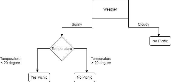
The flow chart can be explained as whether a particular day can be used for Picnic. If the weather is cloudy, there won’t be any picnic. On the other hand if the temperature is more than 20 degree, on a sunny day, there won’t be any picnic either. This is a simple intuitive structure of a decision tree.

Some of the advantages of decision trees are:

1. Simple to understand and interpret.
2. Able to handle multi-label problems.
3. Lots of data is not required

Let me now apply decision tree on our car data-set. we will not convert any column to numerical.

from sklearn import tree
clf = tree.DecisionTreeClassifier()
clf = clf.fit(feature_train, label_train)
y_pred = clf.predict(feature_test)

print("Accuracy:",metrics.accuracy_score(label_test, y_pred))

Accuracy: 0.9614643545279383

from sklearn.metrics import confusion_matrix
import seaborn as sns

conf_matrix = confusion_matrix(label_test, y_pred)
sns.heatmap(conf_matrix, annot=True,cmap='Blues')

We can find out that using decision tree, the accuracy has increased further. Now I will move on to random forest and implement it.

Random Forest

Random forests is an ensemble learning method for classification, regression and other tasks that operates by constructing a lot of decision trees at training time and outputting the class that is the mode of the classes ( for classification task) or mean prediction ( for regression) of the individual.

For example, given a data-set in binary classification task, a random forest will construct 5 different decision trees(DT). Each decision tree predicts that a particular observation belogs to class A or B. Suppose, 3 DT predicts, the observation belongs to class A and 2 DT predicts, that it belongs to class B. The final prediction will be that the observation belongs to class A, because of majority votes.

Random Forest can be used to find the importance of variables. Let me now implement it in our car data-set.

from sklearn.ensemble import RandomForestClassifier

clf = RandomForestClassifier()
clf = clf.fit(feature_train, label_train)
y_pred = clf.predict(feature_test)

print("Accuracy:",metrics.accuracy_score(label_test, y_pred))

Accuracy: 0.9614643545279383

from sklearn.metrics import confusion_matrix
import seaborn as sns

conf_matrix = confusion_matrix(label_test, y_pred)
sns.heatmap(conf_matrix, annot=True,cmap='Blues')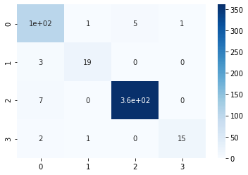

import matplotlib.pyplot as plt

importances = clf.feature_importances_
std = np.std([tree.feature_importances_ for tree in clf.estimators_],
             axis=0)
indices = np.argsort(importances)[::-1]


print("Feature ranking:")

for feat, importance in zip(feature.columns, clf.feature_importances_):
    print('feature: {f}, importance: {i}'.format(f=feat, i=importance))


plt.figure()
plt.title("Feature importances")
plt.bar(range(feature_train.shape[1]), importances[indices],
        color="r", yerr=std[indices], align="center")
plt.xticks(range(feature_train.shape[1]), indices)
plt.xlim([-1, feature_train.shape[1]])
plt.show()

Feature ranking:
feature: buying_price, importance: 0.15805893468088125
feature: maintenance_price, importance: 0.14284411023417876
feature: doors, importance: 0.06261586615016933
feature: person, importance: 0.23607380372770673
feature: luggage_boot, importance: 0.09643509879528141
feature: safety, importance: 0.3039721864117825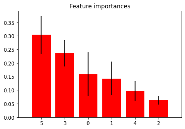

From the above code, we got to know that safety is the most important feature for classification. Now we will move into implementing Naive Bayes.

Naive Bayes

Naive Bayes is a technique for constructing classifiers. There is no single algorithm for training classifiers, but a family of algorithms based on a common principle: all naive Bayes classifiers makes an assumption that value of a particular feature is independent of value of others, given the class . For example, a fruit may be considered to be an orange if it is orange in colour, round, and about 10 cm in diameter. A naive Bayes classifier considers each of the features to contribute independently to the probability, that this fruit is an apple, regardless of any possible correlations between the color, roundness, and diameter features.

Naive Bayes classifiers requires very small amount of data and are majorly used in text classification. But in this blog, I will implement it in our car data-set and look how it performs.

from sklearn.naive_bayes import GaussianNB

gnb = GaussianNB()
gnb = gnb.fit(feature_train, label_train)
y_pred = gnb.predict(feature_test)

print("Accuracy:",metrics.accuracy_score(label_test, y_pred))

Accuracy: 0.7822736030828517

from sklearn.metrics import confusion_matrix
import seaborn as sns

conf_matrix = confusion_matrix(label_test, y_pred)
sns.heatmap(conf_matrix, annot=True,cmap='Blues')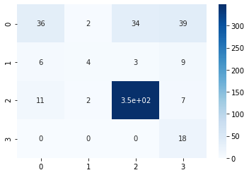

We can see that the Naive Bayes model didn’t perform well in this task, but we got an understanding, how to implement it using scikit-learn. Nex we will move on to implementing Support Vector Machine on this data-set and check how it performs.

Support Vector Machine(SVM)

Support Vector Machine is a supervised machine learning algorithm that is used for both regression and classification. Generally it is used for classification task. In SVM, we start by plotting each data point in n-dimensional space. After plotting the data points, a hyper-plane needs to be found that classifies the data-points according to their labels. The hyper-plane must be constructed in such a way that distance between nearest data-point is maximum.

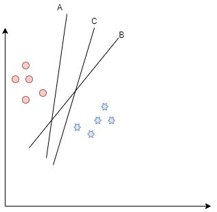
In the above diagram, there are two classes, and we have drawn 3 hyper-planes. From the 3 hyper-planes, it is clear that hyper-plane A is close to red dots, while C is closer to blue stars. So we have to choose B as our required hyper-plane because it differentiates the two class pretty well and nearest distance from both classes is maximum. This is the intuition, how SVM works. Now let me apply it on our data-set.

from sklearn import svm

clf = svm.SVC()
clf = clf.fit(feature_train, label_train)
y_pred = clf.predict(feature_test)

print("Accuracy:",metrics.accuracy_score(label_test, y_pred))

Accuracy: 0.9229287090558767

from sklearn.metrics import confusion_matrix
import seaborn as sns

conf_matrix = confusion_matrix(label_test, y_pred)
sns.heatmap(conf_matrix, annot=True,cmap='Blues')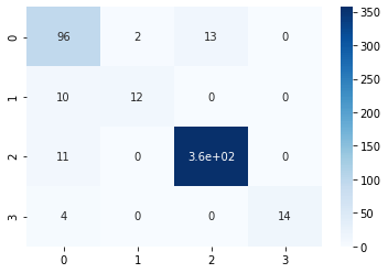

We can see that the SVM model has performed pretty well but not good enough, like the tree based models. Now let us move on to our last and final topic, XG-Boost.

XG-Boost

XG-Boosting is another ensemble based algorithm that learns from “weak learners”. It is one of the newest algorithm and has proved to be highly efficient and fast. In boosting, individual models are not built on completely random subsets of data but sequentially by putting more weight on instances with wrong predictions and high errors. Just like Gradient Descent, it learns from previous mistakes. For example, for a particular observation, the predicted result and the actual result is compared. After comparison, the partial derivative of the loss function is calculated and the weights are adjusted accordingly. I will write about Neural Networks and Gradient Descent in my next blog, and it will be much detailed.

I will implement Gradient Boosting on our car data-set. Before that I will convert data types of “doors” and “person” column to int64.

feature_train['doors'] = pd.to_numeric(feature_train['doors'])
feature_train['person'] = pd.to_numeric(feature_train['person'])
feature_test['doors'] = pd.to_numeric(feature_test['doors'])
feature_test['person'] = pd.to_numeric(feature_test['person'])

from xgboost import XGBClassifier

clf = XGBClassifier()


clf = clf.fit(feature_train, label_train)
y_pred = clf.predict(feature_test)

print("Accuracy:",metrics.accuracy_score(label_test, y_pred))

Accuracy: 0.9884393063583815

from sklearn.metrics import confusion_matrix
import seaborn as sns

conf_matrix = confusion_matrix(label_test, y_pred)
sns.heatmap(conf_matrix, annot=True,cmap='Blues')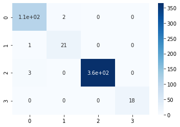

It is quite evident, how powerful xg-boost is and how accurate results can be predicted using this algorithm.

Final Thoughts

We have covered a lots of algorithm in this blog and implemented all of them in python.Readers can take different other data-set and try implementing all the algorithms to have a better understanding of the concepts. Hyper-parameter tuning can also be tested. We saw xg-boost algorithm produced the most accurate results in our car data-set. Supervised learning for classification is a vast field of research and lots of research is going on in the field of Neural Networks and my next blog is about detailed working of it. If you have any doubts, feel free to comment I will get back explaining the solution.