Unsupervised Learning in Python

Hello World, here I am with my new blog and this is about Unsupervised learning in Python. Previously I wrote about Supervised learning methods such as Linear Regression and Logistic regression. In this blog, I am going to discuss about two of the most important methods in unsupervised learning i.e., Principal Component Analysis and Clustering.

Unsupervised learning refers to the fact that the data in use, is not labeled manually as in Supervised learning methods. It looks for previously undetected pattern without any human supervision. In supervised learning, we label data-points as belonging to a class. Hence it is easier for an algorithm to learn from the labelled data. In case of unsupervised learning the data points are grouped as belonging to a cluster based on similarity. Similarity can be measured by plotting a data-point in n-dimensional vector space and finding euclidean distance between data-points. The less the distance, the more similar they are.

Challenges in Unsupervised learning

1. Unsupervised learning is harder in comparison to Supervised learning as there is no annotated data, so the algorithms need to be such that it understands the pattern.
2. We cannot validate the results from Unsupervised learning since no labelled data is present.

Advantages of Unsupervised learning

1. No manual labeling required for annotating huge amount of data
2. We don’t know, into how many classes the data is actually divided.
3. Principal Component Analysis reduces the dimension of large data-set, thus helping in less computation.

Principal Component Analysis(PCA)

Large data-sets are widespread in many sectors. In order to analyse and interpret such data-sets, methods are required to significantly reduce the dimensionality in an interpretable way, such that most of the information is preserved. Many techniques have been developed, but principal component analysis (PCA) is one of the oldest and widely used. Its idea is simple, reduce the dimensionality of a dataset, on the other hand, preserving as much ‘variability’ (i.e. statistical information) as possible.

I will not discuss about working of PCA and how its algorithm works, but straight dive into implementing it in python. I will apply this to a large data-set and check, how it can significantly reduce the dimensionality of it. Let me start by importing necessary packages

import pandas as pd
import numpy as np

I will be working with Breast Cancer data-set. The data-set has 9 feature columns. We will reduce the 9 columns to 3 principal components and understand how much of the information is retained by the 3 principal components.

dataset = pd.read_csv('breast_cancer_dataset.csv')
dataset= dataset.rename(columns={'clump_thickness': 'clumpThickness',
                                'uniformity_of_cell_size': 'cellSize',
                                'uniformity_of_cell_shape':'cellShape',
                                'marginal_adhesion': 'marginalAdhesion',
                                'single_epithelial_cell_size':'singleECellSize'})
dataset.shape

(569, 10)

The data-set has 569 rows and 10 columns.

Let me look at random 5 data from the data-set

dataset.sample(5)

	clumpThickness	cellSize	cellShape	marginalAdhesion	singleECellSize	bare_nuclei	bland_chromatin	normal_nucleoli	mitosis	class
243	1	1	1	1	2	5	5	1	1	2
304	8	3	4	9	3	10	3	3	1	4
21	10	5	5	3	6	7	7	10	1	4
180	1	1	1	1	1	1	3	1	1	2
487	10	10	10	10	6	10	8	1	5	4

dataset.dtypes

clumpThickness      int64
cellSize            int64
cellShape           int64
marginalAdhesion    int64
singleECellSize     int64
bare_nuclei         int64
bland_chromatin     int64
normal_nucleoli     int64
mitosis             int64
class               int64
dtype: object

We have a data-set having all numerical columns. PCA works good for numerical columns and it is not advisable to use PCA with categorical data. Let me check the data-set description using the describe function.

dataset.describe()

	clumpThickness	cellSize	cellShape	marginalAdhesion	singleECellSize	bare_nuclei	bland_chromatin	normal_nucleoli	mitosis	class
count	569	569	569	569	569	569	569	569	569	569
mean	4.539543	3.184534	3.265378	2.845343	3.298770	-2632.518453	3.490334	2.989455	1.637961	2.731107
std	2.896501	3.002236	2.955935	2.873626	2.304775	16035.653408	2.324925	3.091315	1.773941	0.964018
min	1.000000	1.000000	1.000000	1.000000	1.000000	-100000.000000	1.000000	1.000000	1.000000	2.000000
25%	2.000000	1.000000	1.000000	1.000000	2.000000	1.000000	2.000000	1.000000	1.000000	2.000000
50%	4.000000	1.000000	2.000000	1.000000	2.000000	1.000000	3.000000	1.000000	1.000000	2.000000
75%	6.000000	5.000000	5.000000	4.000000	4.000000	8.000000	5.000000	4.000000	1.000000	4.000000
max	10.000000	10.000000	10.000000	10.000000	10.000000	10.000000	10.000000	10.000000	10.000000	4.000000

We can clearly see that there are no missing values but bare_nuclei has minimum value of -100000 which is not normal. So I will replace -100000 with 1. So lets so that.

dataset = dataset.replace(-100000, 1)
dataset.describe()

	clumpThickness	cellSize	cellShape	marginalAdhesion	singleECellSize	bare_nuclei	bland_chromatin	normal_nucleoli	mitosis	class
count	569	569	569	569	569	569	569	569	569	569
mean	4.539543	3.184534	3.265378	2.845343	3.298770	3.711775	3.490334	2.989455	1.637961	2.731107
std	2.896501	3.002236	2.955935	2.873626	2.304775	3.713017	2.324925	3.091315	1.773941	0.964018
min	1.000000	1.000000	1.000000	1.000000	1.000000	1.000000	1.000000	1.000000	1.000000	2.000000
25%	2.000000	1.000000	1.000000	1.000000	2.000000	1.000000	2.000000	1.000000	1.000000	2.000000
50%	4.000000	1.000000	2.000000	1.000000	2.000000	1.000000	3.000000	1.000000	1.000000	2.000000
75%	6.000000	5.000000	5.000000	4.000000	4.000000	8.000000	5.000000	4.000000	1.000000	4.000000
max	10.000000	10.000000	10.000000	10.000000	10.000000	10.000000	10.000000	10.000000	10.000000	4.000000

We have replaced the value. Now I will convert the target variable i.e., ‘class’ into categorical variable where 2 refers to benign and 4 to malignant. I will separate the data-set into feature and target and finally perform standardization to standardize the features, since it is required for PCA. Lets do that.

dataset['class'] = dataset['class'].astype('category')
dataset.dtypes

clumpThickness         int64
cellSize               int64
cellShape              int64
marginalAdhesion       int64
singleECellSize        int64
bare_nuclei            int64
bland_chromatin        int64
normal_nucleoli        int64
mitosis                int64
class               category
dtype: object

feature = dataset.iloc[:,:-1]
feature.sample(5)

	clumpThickness	cellSize	cellShape	marginalAdhesion	singleECellSize	bare_nuclei	bland_chromatin	normal_nucleoli	mitosis
387	5	3	3	2	3	1	3	1	1
388	2	1	1	1	2	1	2	2	1
295	5	5	7	8	6	10	7	4	1
37	6	2	1	1	1	1	7	1	1
289	5	6	6	8	6	10	4	10	4

target = dataset['class']
target.sample(5)

314    2
110    2
52     4
393    2
338    2
Name: class, dtype: category
Categories (2, int64): [2, 4]

from mlxtend.preprocessing import standardize

feature = standardize(feature, columns=feature.columns)
feature.sample(5)

	clumpThickness	cellSize	cellShape	marginalAdhesion	singleECellSize	bare_nuclei	bland_chromatin	normal_nucleoli	mitosis
214	1.886849	2.272127	2.280344	2.491957	-0.129745	1.695052	2.802410	0.974729	-0.359946
23	1.195754	0.271858	0.587343	-0.642730	-0.564008	-0.730985	1.510911	0.003414	-0.359946
9	-0.186438	-0.394898	-0.767057	-0.642730	-0.564008	-0.730985	-0.641589	-0.644129	-0.359946
318	-1.223082	-0.728276	-0.767057	-0.642730	0.738782	-0.730985	-0.211089	-0.644129	-0.359946
224	1.886849	0.605237	0.587343	1.098763	-0.129745	1.695052	1.510911	1.946044	0.204267

Now that we have standardized the data-set, we will apply PCA

from sklearn.decomposition import PCA
pcaData = PCA(n_components=3)
principalComps = pcaData.fit_transform(feature)
principalDataset = pd.DataFrame(data = principalComps
             , columns = ['p_comp1', 'p_comp2','p_comp3'])

principalDataset.sample(5)

	p_comp1	p_comp2	p_comp3
202	-1.963079	0.091061	0.569509
384	-2.149096	0.269625	0.139878
92	-1.644486	-0.054447	-0.246690
54	2.679463	-0.995198	-0.594913
217	-1.963079	0.091061	0.569509

We have converted the entire data-set into a data-set with only 3 features i.e., Principal Components. Lets checkout how the principal components can explain the variance, i.e., information retained by 3 principal components.

pcaData.explained_variance_ratio_

array([0.6501069 , 0.08621319, 0.06142388])

From the above code, we can understand that the 1st principal component has 65% of the information, while 2nd and 3rd has 8% and 6% information, respectively.

We can use this principal components as features and develop our classification or regression models.

PCA is very sensitive to outliers and so, outliers must be detected and handled. PCA creates variables that are linear combinations of the original variables. The new variables have the orthogonal property. PCA transformation can be helpful as pre-processing step before clustering

Now that we have understood how to implement PCA in python, we will look at clustering and understand how to implement clustering in python.

Clustering

Clustering is a very important topic in machine-learning, where we can can create groups of data from a sample, having similar values. Annotating large data-sets is a very hectic task and needs extensive time and effort to accomplish. Clustering comes to the rescue and can be implemented easily in python. There are lots of clustering algorithms but I will discuss about K-Means Clustering and Hierarchical Clustering. K-means clustering is centroid based, while Hierarchical clustering is connectivity based.

K-Means Clustering

K-Means Clustering is an algorithm that falls under the category of centroid-based clustering. K-Means clustering can be used in Customer Segmentation, Recommendation Engine,etc. In K-means clustering, each observation belongs to a particular cluster, which has the nearest mean(cluster centroid). Euclidean distance is used to measure the distance and variance is used to measure scatter between clusters. The intra-cluster variation, or Within-cluster sum of squares(WSS) needs to be minimum and Inter-Cluster variance needs to be maximum.

At first, we have to choose, into how many clusters, the data-set will be divided into. Suppose we select k clusters, so k points will be randomly assigned as centroid in vector space. Now distance between each data points and the k centroids are calculated. The data points closer to the centroid are clubbed as a single cluster. Now in next iteration, the new centroid is calculated for each clusters formed, and the data points are clubbed into clusters. The process repeats untill there is no change in the centroid formed. Finally, similar data points can be found as clusters.

Let us implement K-means clustering in Python.

I will be using the above data-set excluding the target variable. Next we will use elbow curve to choose number of clusters and check whether there are 2 clusters, since there are two classes in the original data-set.

Elbow curve helps us to determine optimal number of clusters. The location of the bend helps to determine the optimal number of clusters.

from sklearn.cluster import KMeans
from yellowbrick.cluster import KElbowVisualizer

clusteringDataset = dataset.iloc[: ,:-1]

model = KMeans()
visualizer = KElbowVisualizer(model, k=(1,8))

visualizer.fit(clusteringDataset)        
visualizer.show()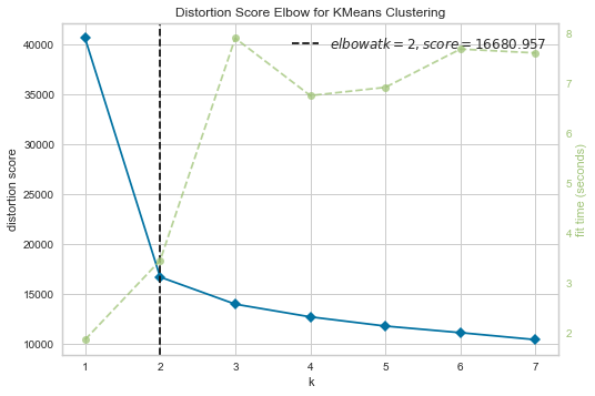 

We can clearly see that we should choose 2 clusters for this data-set. Lets Apply K-means clustering now on the data-set and visualize the result.

import matplotlib.pyplot as plt
kmeans = KMeans(n_clusters=2)
kmeans.fit(clusteringDataset)
y_kmeans = kmeans.predict(clusteringDataset)

plt.scatter(clusteringDataset.iloc[:, 0], clusteringDataset.iloc[:, 1], c=y_kmeans, s=50, cmap='viridis')

centers = kmeans.cluster_centers_
plt.scatter(centers[:, 0], centers[:, 1], c='red', s=200, alpha=0.5)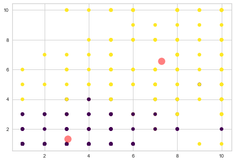

We understood how to use k-means clustering and how to choose optimum number of clusters from elbow curve. K-means clustering has got lot of uses The next topic is about Hierarchical clustering.

Hierarchical clustering

Hierarchical Clustering is another clustering technique, which starts by refering individual observations as a cluster. Then it follows two steps:

1. Identify closest data point

2. Merge them as cluster

The output from Hierarchical clustering is a dendrogram.

For applying and visualizing hierarchical clustering, lets generate a simple data-set. The data-set has two columns, since two-dimensional data is easy to visualize.

np.random.seed(4715) 
a = np.random.multivariate_normal([10, 30], [[3, 1], [1, 4]], size=[50,])
b = np.random.multivariate_normal([5, 20], [[3, 1], [1, 4]], size=[20,])
X = np.concatenate((a, b),)
plt.scatter(X[:,0], X[:,1])
plt.show()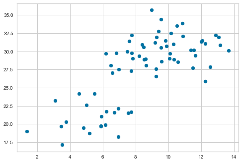

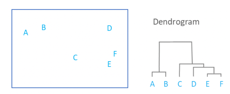
We have created the data-set and plotted a scatterplot. Let us visualize the dendrogram. A dendrogram is a structure that shows the hierarchical relationship between data. It is most commonly created as an output of hierarchical clustering. The main use of a dendrogram is to find out the best way to allocate data-points to clusters. In the dendrogram below, the height of the dendrogram indicates the order in which the clusters were joined. A more informative dendrogram can be generated where the heights reflect the distance between the clusters as is shown below. In this case, the dendrogram shows us the big difference between clusters is between the cluster of A and B versus that of C, D, E, and F.

from scipy.cluster.hierarchy import dendrogram, linkage
from matplotlib import pyplot as plt

linked = linkage(X, 'single')

plt.figure(figsize=(10, 7))
dendrogram(linked,
            orientation='top',            
            distance_sort='descending',
            show_leaf_counts=True)
plt.show()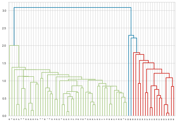

From the dendrogram, we can understand that there are basically 2 clusters. Now let me perform Hierarchical Clustering using 2 clusters.

from sklearn.cluster import AgglomerativeClustering

cluster = AgglomerativeClustering(n_clusters=2, affinity='euclidean', linkage='ward')
cluster.fit_predict(X)
plt.scatter(X[:,0],X[:,1], c=cluster.labels_, cmap='rainbow')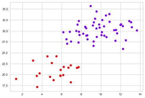

In the above diagram, we got to visualize the two clusters. Hierarchical clustering is preferred when the data is small. When the data-set is large enough, K-means clustering will be helpful, as it is more robust.

Final Words – Unsupervised Learning in Python

In this blog, I have discussed about PCA and about two of the most important Clustering technique. We found out how easy it is to implement them in Python and how to generate different visualizations. I will expect my readers to dive deeper into these concepts and to perform hyper-parameter tuning for better results. I will also like them to implement these algorithms in real life data and gain insights from that. In my next blog, I will be writing about Classification models such as K-NN, Naive Bayes, Random Forest, etc. If you find my blogs useful, please let me know in the comments below.