Regression Analysis using Python

I have been working as a data analytics professional for 3 years now, and I think Linear regression is the building block for anyone, who are entering this data driven world. So, what makes linear regression such an important algorithm? I will explain everything about regression analysis in detail and provide python code along with the explanations. So just grab a coffee and please read it till the end.

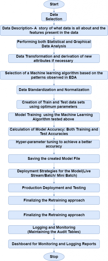
Linear Regression is one of the most fundamental algorithms in the Machine Learning world. It is the door to the magical world ahead. But before proceeding with the algorithm, let’s first discuss the life cycle of any machine learning model. This diagram explains the creation of a Machine Learning model from scratch and then taking the same model further with hyper-parameter tuning to increase its accuracy. A typical life cycle diagram for a machine learning model looks like:

What is Regression Analysis?

Regression is the process of predicting a Label based on the features at hand. For example, the relationship between stock prices of a company and various factors like customer reputation, company annual performance, etc. can be studied using regression.

Regression analysis is an important tool for analysing and modelling data. Here, we fit a curve to the data points, in such a manner that the differences between the distance of the actual data points from the plotted curve is the least. The topic will be explained in detail in the coming sections.

The use of Regression

Regression analyses the relationship between two or more features. Let’s take an example:

Let’s suppose we want to make an application which predicts the chances of admission a student to a foreign university. In that case, the

The benefits of using Regression analysis are as follows:

• It shows the significant relationships between the Label (dependent variable) and the features (independent variable).
• It shows the extent of impact of multiple independent variables on the dependent variable.
• It can also measure these effects even if the variables are on a different scale.

These features enable the data scientists to find the best set of independent variables for predictions.

Linear Regression

Linear Regression is the most important and widely known Machine Learning Algorithms which people start with. A linear regression model consists of:

• Discreet/continuous independent variables
• A best-fit regression line
• Continuous dependent variable. The equation of the Linear Regression is: Y=a+b*X + e where, a is the intercept, b is the slope of the line, and e is the error term. The equation above is used to predict the value of the target based on the given predictors.

The Problem statement:

This data is about the amount spent on advertising through different channels like TV, Radio and Newspaper. The goal is to predict how the expense on each channel affects the sales and is there a way to optimize that sale?

# necessary Imports
import pandas as pd
import matplotlib.pyplot as plt
import pickle
% matpllotlib inline

data= pd.read_csv('Advertising.csv') # Reading the data file
data.head() # checking the first five rows from the dataset

	Unnamed: 0	TV	radio	newspaper	sales
0	1	230.1	37.8	69.2	22.1
1	2	44.5	39.3	45.1	10.4
2	3	17.2	45.9	69.3	9.3
3	4	151.5	41.3	58.5	18.5
4	5	180.8	10.8	58.4	12.9

What are the features?

• TV: Dollars spent for advertising on TV for a single product in a given market (in thousands of dollars)
• Radio: Dollars spent for advertising on Radio
• Newspaper: Dollars spent for advertising on Newspaper

What is the response?

• Sales: Sale of a single product in a given market (in thousands)

data.shape

(200, 5)

data.info() # printing the summary of the dataframe

<class 'pandas.core.frame.DataFrame'>
RangeIndex: 200 entries, 0 to 199
Data columns (total 5 columns):
Unnamed: 0    200 non-null int64
TV            200 non-null float64
radio         200 non-null float64
newspaper     200 non-null float64
sales         200 non-null float64
dtypes: float64(4), int64(1)
memory usage: 7.9 KB

data.isna().sum() # finding the count of missing values from different columns

Unnamed: 0    0
TV            0
radio         0
newspaper     0
sales         0
dtype: int64

Now, let’s visualize the relationship between the feature and target column

# visualizing the relationship between features and response using scatterplots
fig, axs = plt.subplots(1, 3, sharey=True)
data.plot(kind='scatter', x='TV', y='sales', ax=axs[0], figsize=(16, 8))
data.plot(kind='scatter', x='radio', y='sales', ax=axs[1])
data.plot(kind='scatter', x='newspaper', y='sales', ax=axs[2])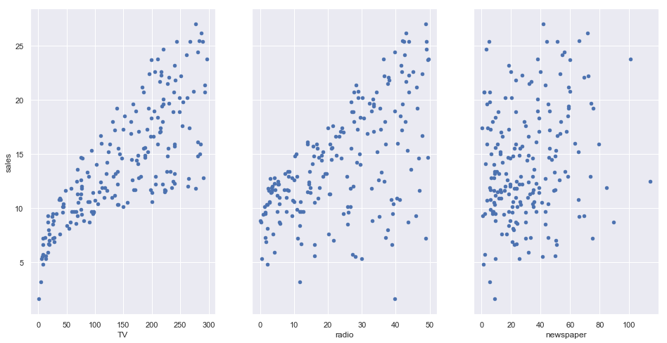

Questions about the data

A generic question shall be: How the company should optimise the spends on advertising to maximise the sales?

More specific questions can come up from this general questions:

1. What’s the relationship between ads and sales?
2. How prominent is that relationship?
3. Which ad types contribute to sales?
4. How each ad contributes to sales?
5. Can sales be predicted given the expense of the advertisement?

We will explore these questions below!

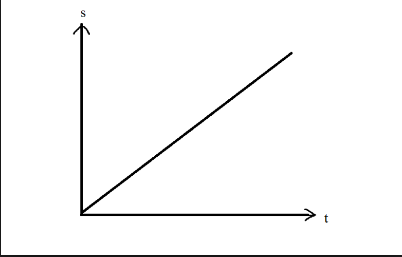
From the relationship diagrams above, it can be observed that there seems to be a linear relationship between the features TV ad, Radio ad and the sales is almost a linear one. A linear relationship typically looks like:

Hence, we can build a model using the Linear Regression Algorithm.

Simple Linear Regression

Simple Linear regression is a method for predicting a target variable using a single feature (“input variable”). The mathematical equation is:

?=β0+β1x

What do terms represent?

• ? is the target variable
• ? is the feature
• β1 is the coefficient of x
• β0 is the intercept

β0 and β1 are the model coefficients. To create a model, we should “learn” the values of the coefficients. And once we have the value of the coefficients, we can use the model to predict the Sales!

Multiple Linear Regression

Till now, we have created the model based on only one feature. Now, we’ll include multiple features and create a model to see the relationship between those features and the label column. This is called Multiple Linear Regression.

?=?0+?1?1+…+????

Each ? represents different features, and each feature has its own co-efficient. In this case:

?=?0+?1×??+?2×?????+?3×?????????

Let’s use Statsmodels to estimate these coefficients

# create X and y
feature_cols = ['TV', 'radio', 'newspaper']
X = data[feature_cols]
y = data.sales

lm = LinearRegression()
lm.fit(X, y)

# print intercept and coefficients
print(lm.intercept_)
print(lm.coef_)

2.9388893694594085
[ 0.04576465  0.18853002 -0.00103749]

How do we interpret these coefficients? If we look at the coefficients, the coefficient for the newspaper spends is negative. It means that the money spent for newspaper advertisements is not contributing in a positive way to the sales.

A lot of the information is available in the model summary output:

l_m = smf.ols(formula='sales ~ TV + radio + newspaper', data=data).fit()
l_m.conf_int()
l_m.summary()

Dep. Variable:	sales	R-squared:	0.897
Model:	OLS	Adj. R-squared:	0.896
Method:	Least Squares	F-statistic:	570.3
Date:	Fri, 27 Dec 2019	Prob (F-statistic):	1.58e-96
Time:	20:12:27	Log-Likelihood:	-386.18
No. Observations:	200	AIC:	780.4
Df Residuals:	196	BIC:	793.6
Df Model:	3
Covariance Type:	nonrobust

	coef	std err	t	P>|t|	[0.025	0.975]
Intercept	2.9389	0.312	9.422	0.000	2.324	3.554
TV	0.0458	0.001	32.809	0.000	0.043	0.049
radio	0.1885	0.009	21.893	0.000	0.172	0.206
newspaper	-0.0010	0.006	-0.177	0.860	-0.013	0.011

Omnibus:	60.414	Durbin-Watson:	2.084
Prob(Omnibus):	0.000	Jarque-Bera (JB):	151.241
Skew:	-1.327	Prob(JB):	1.44e-33
Kurtosis:	6.332	Cond. No.	454.

What are the things to be learnt from this summary?

• TV and Radio have positive p-values, whereas Newspaper has a negative one. Hence, we can reject the null hypothesis for TV and Radio that there is no relation between those features and Sales, but we fail to reject the null hypothesis for Newspaper that there is no relationship between newspaper spends and sales.
• The expenses on bot TV and Radio ads are positively associated with Sales, whereas the expense on newspaper ad is slightly negatively associated with the Sales.
• This model has a higher value of R-squared (0.897) than the previous model, which means that this model explains more variance and provides a better fit to the data than a model that only includes the TV.

Feature Selection

How do I decide which features have to be included in a linear model? Here’s one idea:

• Try different models, and keep only the predictors, if they have small p-values.
• Check if the R-squared value goes up when you add new predictors to the model.

What are the drawbacks in this approach? -If the underlying assumptions for creating a Linear model(the features being independent) are violated(which usually is the case),p-values and R-squared values are less reliable.

• Using a p-value cutoff of 0.05 means that adding 100 predictors to a model that are pure noise, still 5 of them (on average) will be counted as significant.
• R-squared is susceptible to model over-fitting, and thus there is no guarantee that a model with a high R-squared value will generalize. Following is an example:

#include only TV and Radio in the model
l_m = smf.ols(formula='sales ~ TV + radio', data=data).fit()
l_m.rsquared

0.8971942610828956

# add Newspaper to the model (which is believed to have no association with Sales)
l_m = smf.ols(formula='sales ~ TV + radio + newspaper', data=data).fit()
l_m.rsquared

0.8972106381789522

Selecting the model with the highest value of R-squared is not a correct approach as the value of R-squared shall always increase whenever a new feature is taken for consideration even if the feature is unrelated to the response.

The alternative is to use adjusted R-squared which penalizes the model complexity (to control over-fitting), but this again generally under-penalizes complexity.

a better approach to feature selection is Cross-validation. It provides a more reliable way to choose which of the created models will best generalize as it better estimates of out-of-sample error. An advantage is that the cross-validation method can be applied to any machine learning model and the scikit-learn package provides extensive functionality for that.

Multi- Collinearity

Origin of the word: The word multi-collinearity consists of two words:Multi, meaning multiple, and Collinear, meaning being linearly dependent on each other.

For e.g., Let’s consider this equation ?+?=1 => ?=1−?

It means that ‘b’ can be represented in terms of ‘a’ i.e., if the value of ‘a’ changes, automatically the value of ‘b’ will also change. This equation denotes a simple linear relationship among two variables.

Definition: The purpose of executing a Linear Regression is to predict the value of a dependent variable based on certain independent variables.

So, when we perform a Linear Regression, we want our dataset to have variables which are independent i.e., we should not be able to define an independent variable with the help of another independent variable because now in our model we have two variables which can be defined based on a certain set of independent variables which defeats the entire purpose.

• Multi-collinearity is the statistical term to represent this type of a relation among the independent variable- when the independent variables are not so independent?.
• We can define multi-collinearity as the situation where the independent variables (or the predictors) have strong correlation among themselves.

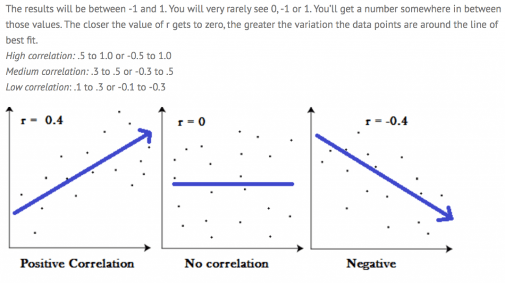
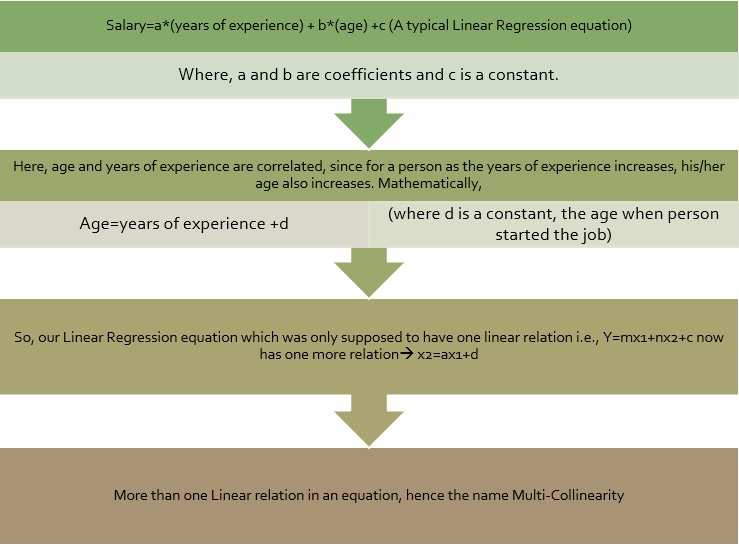
The mathematical flow for multicollinearity can be shown as:

Why Should We Care About Multi-Collinearity?

• The coefficients in a Linear Regression model represent the extent of change in Y when a certain x (amongst X1,X2,X3…) is changed keeping others constant. But, if x1 and x2 are dependent, then this assumption itself is wrong that we are changing one variable keeping others constant as the dependent variable will also be changed. It means that our model itself becomes a bit flawed.
• We have a redundancy in our model as two variables (or more than two) are trying to convey the same information.
• As the extent of the collinearity increases, there is a chance that we might produce an over-fitted model. An over-fitted model works well with the test data but its accuracy fluctuates when exposed to other data sets.
• Can result in a Dummy Variable Trap.

Detection

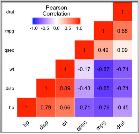
• Correlation Matrices and Plots: for correlation between all the X variables. This plot shows the extent of correlation between the independent variable. Generally, a correlation greater than 0.9 or less than -0.9 is to be avoided.

Variance Inflation Factor: Regression of one X variable against other X variables.

VIF=1/(1−????????)

      The VIF factor, if greater than 10 shows extreme correlation between the variables and then we need to take care of the correlation.

Remedies for Multicollinearity

• Do Nothing: If the Correlation is not that extreme, we can ignore it. If the correlated variables are not used in solving our business question, they can be ignored.
• Remove One Variable: Like in dummy variable trap
• Combine the correlated variables: Like creating a seniority score based on Age and Years of experience
• Principal Component Analysis

#Let's start with importing necessary libraries

import pandas as pd 
import numpy as np 
from sklearn.preprocessing import StandardScaler 
from sklearn.linear_model  import LinearRegression,LassoCV, Lasso
from sklearn.model_selection import train_test_split
import statsmodels.api as sm 
import matplotlib.pyplot as plt
import seaborn as sns
sns.set()

# Let's create a function to create adjusted R-Squared
def adj_r2(x,y):
    r2 = regression.score(x,y)
    n = x.shape[0]
    p = x.shape[1]
    adjusted_r2 = 1-(1-r2)*(n-1)/(n-p-1)
    return adjusted_r2

data =pd.read_csv('Admission_Prediction.csv')
data.head()

	Serial No.	GRE Score	TOEFL Score	University Rating	SOP	LOR	CGPA	Research	Chance of Admit
0	1	337.0	118.0	4.0	4.5	4.5	9.65	1	0.92
1	2	324.0	107.0	4.0	4.0	4.5	8.87	1	0.76
2	3	NaN	104.0	3.0	3.0	3.5	8.00	1	0.72
3	4	322.0	110.0	3.0	3.5	2.5	8.67	1	0.80
4	5	314.0	103.0	2.0	2.0	3.0	8.21	0	0.65

data.describe(include='all')

	Serial No.	GRE Score	TOEFL Score	University Rating	SOP	LOR	CGPA	Research	Chance of Admit
count	500.000000	485.000000	490.000000	485.000000	500.000000	500.00000	500.000000	500.000000	500.00000
mean	250.500000	316.558763	107.187755	3.121649	3.374000	3.48400	8.576440	0.560000	0.72174
std	144.481833	11.274704	6.112899	1.146160	0.991004	0.92545	0.604813	0.496884	0.14114
min	1.000000	290.000000	92.000000	1.000000	1.000000	1.00000	6.800000	0.000000	0.34000
25%	125.750000	308.000000	103.000000	2.000000	2.500000	3.00000	8.127500	0.000000	0.63000
50%	250.500000	317.000000	107.000000	3.000000	3.500000	3.50000	8.560000	1.000000	0.72000
75%	375.250000	325.000000	112.000000	4.000000	4.000000	4.00000	9.040000	1.000000	0.82000
max	500.000000	340.000000	120.000000	5.000000	5.000000	5.00000	9.920000	1.000000	0.97000

data['University Rating'] = data['University Rating'].fillna(data['University Rating'].mode()[0])
data['TOEFL Score'] = data['TOEFL Score'].fillna(data['TOEFL Score'].mean())
data['GRE Score']  = data['GRE Score'].fillna(data['GRE Score'].mean())

data.describe()

	Serial No.	GRE Score	TOEFL Score	University Rating	SOP	LOR	CGPA	Research	Chance of Admit
count	500.000000	500.000000	500.000000	500.000000	500.000000	500.00000	500.000000	500.000000	500.00000
mean	250.500000	316.558763	107.187755	3.118000	3.374000	3.48400	8.576440	0.560000	0.72174
std	144.481833	11.103952	6.051338	1.128993	0.991004	0.92545	0.604813	0.496884	0.14114
min	1.000000	290.000000	92.000000	1.000000	1.000000	1.00000	6.800000	0.000000	0.34000
25%	125.750000	309.000000	103.000000	2.000000	2.500000	3.00000	8.127500	0.000000	0.63000
50%	250.500000	316.558763	107.000000	3.000000	3.500000	3.50000	8.560000	1.000000	0.72000
75%	375.250000	324.000000	112.000000	4.000000	4.000000	4.00000	9.040000	1.000000	0.82000
max	500.000000	340.000000	120.000000	5.000000	5.000000	5.00000	9.920000	1.000000	0.97000

Now the data looks good and there are no missing values. Also, the first cloumn is just serial numbers, so we don’ need that column. Let’s drop it from data and make it more clean.

data= data.drop(columns = ['Serial No.'])
data.head()

	GRE Score	TOEFL Score	University Rating	SOP	LOR	CGPA	Research	Chance of Admit
0	337.000000	118.0	4.0	4.5	4.5	9.65	1	0.92
1	324.000000	107.0	4.0	4.0	4.5	8.87	1	0.76
2	316.558763	104.0	3.0	3.0	3.5	8.00	1	0.72
3	322.000000	110.0	3.0	3.5	2.5	8.67	1	0.80
4	314.000000	103.0	2.0	2.0	3.0	8.21	0	0.65

Let’s visualize the data and analyze the relationship between independent and dependent variables:

# let's see how data is distributed for every column
plt.figure(figsize=(20,25), facecolor='white')
plotnumber = 1

for column in data:
    if plotnumber<=16 :
        ax = plt.subplot(4,4,plotnumber)
        sns.distplot(data[column])
        plt.xlabel(column,fontsize=20)
        #plt.ylabel('Salary',fontsize=20)
    plotnumber+=1
plt.tight_layout()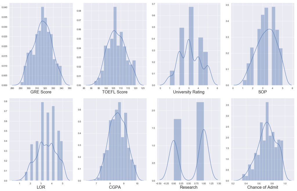

The data distribution looks decent enough and there doesn’t seem to be any skewness. Great let’s go ahead!

Let’s observe the relationship between independent variables and dependent variable.

y = data['Chance of Admit']
X =data.drop(columns = ['Chance of Admit'])

plt.figure(figsize=(20,30), facecolor='white')
plotnumber = 1

for column in X:
    if plotnumber<=15 :
        ax = plt.subplot(5,3,plotnumber)
        plt.scatter(X[column],y)
        plt.xlabel(column,fontsize=20)
        plt.ylabel('Chance of Admit',fontsize=20)
    plotnumber+=1
plt.tight_layout()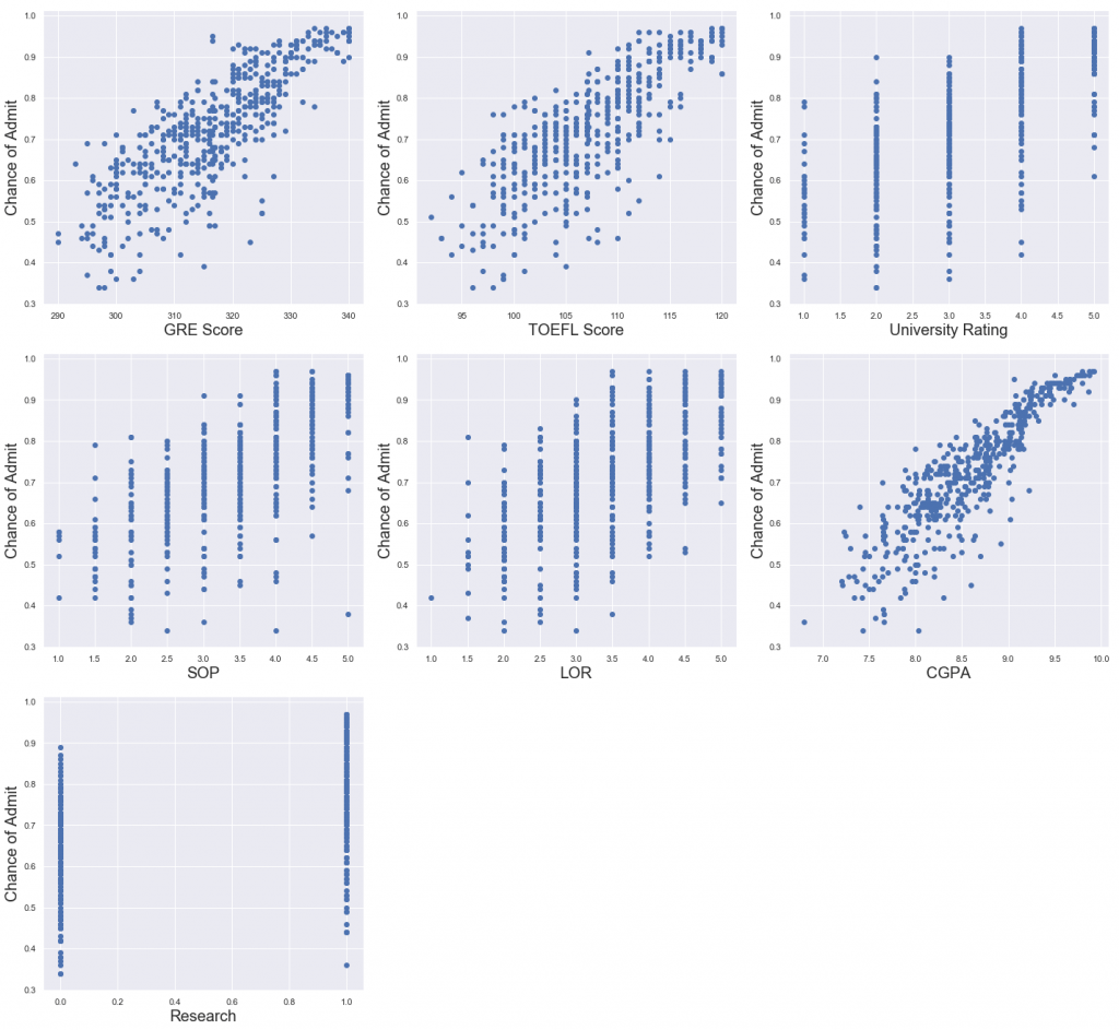

Great, the relationship between the dependent and independent variables look fairly linear. Thus, our linearity assumption is satisfied.

Let’s move ahead and check for multi-collinearity.

scaler =StandardScaler()

X_scaled = scaler.fit_transform(X)

from statsmodels.stats.outliers_influence import variance_inflation_factor
variables = X_scaled

# we create a new data frame which will include all the VIFs
# note that each variable has its own variance inflation factor as this measure is variable specific (not model specific)
# we do not include categorical values for mulitcollinearity as they do not provide much information as numerical ones do
vif = pd.DataFrame()

# here we make use of the variance_inflation_factor, which will basically output the respective VIFs 
vif["VIF"] = [variance_inflation_factor(variables, i) for i in range(variables.shape[1])]
# Finally, I like to include names so it is easier to explore the result
vif["Features"] = X.columns

	VIF	Features
0	4.152735	GRE Score
1	3.793345	TOEFL Score
2	2.517272	University Rating
3	2.776393	SOP
4	2.037449	LOR
5	4.654369	CGPA
6	1.459411	Research

Here, we have the correlation values for all the features. As a thumb rule, a VIF value greater than 5 means a very severe multi-collinearity. We don’t have any variables with VIF greater than 5 , so we are good to go.

Great. Let’s go ahead and use linear regression and see how good it fits our data. But first, let’s split our dataset into train and test.

x_train,x_test,y_train,y_test = train_test_split(X_scaled,y,test_size = 0.25,random_state=355)

regression = LinearRegression()

regression.fit(x_train,y_train)

LinearRegression(copy_X=True, fit_intercept=True, n_jobs=None,
         normalize=False)

# saving the model in local
filename = 'finalized_model.pickle'
pickle.dump(regression, open(filename, 'wb'))

# prediction using the saved model
loaded_model = pickle.load(open(filename, 'rb'))
a=loaded_model.predict(scaler.transform([[300,110,5,5,5,10,1]]))
a

array([0.92190162])

regression.score(x_train,y_train)

0.8415250484247909

adj_r2(x_train,y_train)

0.8385023654247188

Our r2 score is 84.15% and adj r2 is 83.85% for our training set., so looks like we are not being penalized by use of any feature.

Let’s check how well model fits the test data.

Now let’s check if our model is overfitting our data using regularization.

regression.score(x_test,y_test)

0.7534898831471066

adj_r2(x_test,y_test)

0.7387414146174464

So it looks like our model r2 score is less on the test data.

Let’s see if our model is overfitting our training data.

# Lasso Regularization
# LassoCV will return best alpha and coefficients after performing 10 cross validations
lasscv = LassoCV(alphas = None,cv =10, max_iter = 100000, normalize = True)
lasscv.fit(x_train, y_train)

LassoCV(alphas=None, copy_X=True, cv=10, eps=0.001, fit_intercept=True,
    max_iter=100000, n_alphas=100, n_jobs=None, normalize=True,
    positive=False, precompute='auto', random_state=None,
    selection='cyclic', tol=0.0001, verbose=False)

# best alpha parameter
alpha = lasscv.alpha_
alpha

3.0341655445178153e-05

#now that we have best parameter, let's use Lasso regression and see how well our data has fitted before

lasso_reg = Lasso(alpha)
lasso_reg.fit(x_train, y_train)

Lasso(alpha=3.0341655445178153e-05, copy_X=True, fit_intercept=True,
   max_iter=1000, normalize=False, positive=False, precompute=False,
   random_state=None, selection='cyclic', tol=0.0001, warm_start=False)

lasso_reg.score(x_test, y_test)

0.7534654960492284

our r2_score for test data (75.34%) comes same as before using regularization. So, it is fair to say our OLS model did not overfit the data.

So, here in this blog I tried to explain most of the concepts in detail related to Linear regression using python. Please let me know, how you liked this post.I will be writing more blogs related to different Machine Learning as well as Deep Learning concepts. Stay tuned for further updates.