Hello World!!! I am here with a new blog and today’s discussion will be about an important topic in Machine Learning, i.e., Logistic Regression. I will try to explain everything related to logistic regression, in details, with implementation of an use-case in my favorite programming language, Python.

Researchers are often interested in setting up a model to analyze the relationship between predictors (i.e., independent variables) and it’s corresponding response (i.e., dependent variable). Linear regression is commonly used when the target variable is continuous. One assumption of linear models is that the residual errors follow a normal distribution. This assumption fails when the target variable is categorical, so an ordinary linear model is not appropriate. This blog presents a regression model for response variable that is dichotomous–having two categories. Examples are common: whether a survey respondent agrees or disagrees with a statement, whether a plant lives or dies, or whether an individual default on the loan.

In ordinary linear regression, the response variable (Y) is a linear function of the coefficients (B0, B1, etc.) that correspond to the predictor variables (X1, X2, etc.,). A typical model would look like:

Y = B0 + B1*X1 + B2*X2 + B3*X3 + B4*X4 + … + E

For a dichotomous response variable, we could set up a similar linear model to predict individual category memberships if numerical values are used to represent the two categories. Arbitrary values of 0 and 1 are chosen for mathematical convenience. Using the final example, we would assign Y = 1 if an individual defaults on the loan and Y = 0 if he/she doesn’t.

This linear regression model does not work well for quite a few reasons. First, the response values, 1 and 0, are arbitrary,and so modeling the actual values of Y is not exactly of interest. Second, it is the probability that each individual in the population responds with 0 or 1 that we are interested in modeling. For example, we may find that an individual who is married and have children more than two, falls into category who will default on the loan, than an individual who is unmarried. Thus, as number of children increases, the probability of defaulting on the loan also increases.
Thus, we might consider modeling P, the probability, as the target variable. Again, there are problems. Although the general decrease in probability is accompanied by a general increase in number of children, we know that P, like all probabilities, can only fall within the boundaries of 0 and 1. Consequently, it is better to assume that the relationship between X1 and P is sigmoidal (S-shaped), rather than a straight line.

It is possible, however, to find a linear relationship between X1 and function of P. Although a number of functions work, one of the most useful is logit function. It is natural log of the odds that Y is equal to 1, which is simply the ratio of the probability that Y is 1 divided by the probability that Y is 0. The relationship between P and the logit of P itself is sigmoidal in shape. The regression equation that results is:

ln[P/(1-P)] = B0 + B1*X1 + B2*X2 + …

Although the left side of this equation looks intimidating, this way of expressing the probability results in the right side of the equation being linear and familiar to us. This helps us understand the meaning of the regression coefficients. The coefficients can be easily transformed so that their interpretation makes sense.

The logistic regression equation can be extended beyond case of a binary response variable to cases of ordered categories and polytomous categories (more than two categories).

Mathematics behind Logistic Regression

Notation

The problem structure is the classic classification problem. Our data set D is composed of ? samples. Each sample is a tuple containing a feature vector and a label. For any sample ? the feature vector is a ?+1 dimensional column vector denoted by ?? with ? real-valued components known as features. Samples are represented in homogeneous form with the first component equal to 1 : ?0=1 . Vectors are bold-faced. The associated label is denoted ?? and can take only two values: +1 or −1 .

Derivation

Despite the name logistic regression this is actually a probabilistic classification model. It is also a linear model which can be subjected to nonlinear transforms.

All linear models make use of a “signal” ? which is a linear combination of the input vector ? components weighed by the corresponding components in a weight vector ?.

Note that the homogeneous representation (with the 1 at the first component) allows us to include a constant offset using a more compact vector-only notation (instead of ???+?).

Linear classification passes the signal through a harsh threshold:

Linear regression uses the signal directly without modification:

Logistic regression passes the signal through the logistic/sigmoid but then treats the result as a probability:

The logistic function is

There are many other formulas that can achieve a soft threshold such as the hyperbolic tangent, but this function results in some nice simplification.

We say that the data is generated by a noisy target.

With this noisy target we want to learn a hypothesis ℎ(?) that best fits the above noisy target according to some error function.

It’s important to note that the data does not tell you the probability of a label, rather it tells what label the sample has after being generated by the target distribution.

Learning Algorithm

The learning algorithm is how we search the set of possible hypotheses (hypothesis space H) for the best parameterization (in this case the weight vector ?). This search is an optimization problem looking for the hypothesis that optimizes an error measure.

There is no sophisticated, closed-form solution like least-squares linear, so we will use gradient descent instead. Specifically we will use batch gradient descent which calculates the gradient from all data points in the data set.

Luckily, our “cross-entropy” error measure is convex so there is only one minimum. Thus the minimum we arrive at is the global minimum.

Gradient descent is a general method and requires twice differentiability for smoothness. It updates the parameters using a first-order approximation of the error surface.

To learn we’re going to minimize the following error measure using batch gradient descent.

We’ll need the derivative of the point loss function and possibly some abuse of notation.

With the point loss derivative we can determine the gradient of the in-sample error:

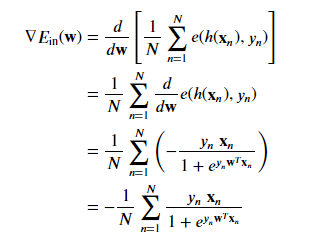
Our weight update rule per batch gradient descent becomes

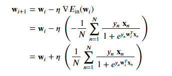
Enough of the theory. Now let us jump straight into the implementation part.

Logistic Regression with scikit-learn

Dataset

The data-set is the affairs dataset that comes with Statsmodels. It is derived from a survey of women in 1974 by Redbook magazine, in which married women were asked about participating in extramarital affairs. More information about the study is available in  1978 paper from the Journal of Political Economy.

Description of Variables

The dataset contains 6366 observations of 9 variables:

• rate_marriage: women’s rating of her marriage (1 = very poor, 5 = very good)
• age: women’s age
• yrs_married: number of years married
• children: number of children
• religious: women’s rating of how religious she is (1 = not religious, 4 = strongly religious)
• educ: level of education (9 = grade school, 12 = high school, 14 = some college, 16 = college graduate, 17 = some graduate school, 20 = advanced degree)
• occupation:occupation of women(1 = student, 2 = farming/semi-skilled/unskilled, 3 = “white collar”, 4 = teacher/nurse/writer/technician/skilled, 5 = managerial/business, 6 = professional with advanced degree)
• occupation_husb: occupation of husband (same coding as above)
• affairs: time spent in extra-marital affairs

Problem Statement

I have decided to treat this as a classification problem by creating a new binary variable affair (if the woman have at least one affair?) and try to predict the classification for each woman.

Import modules

import numpy as np
import pandas as pd
import statsmodels.api as sm
import matplotlib.pyplot as plt
from patsy import dmatrices
from sklearn.linear_model import LogisticRegression
from sklearn.model_selection import train_test_split as split
from sklearn import metrics
from sklearn.model_selection import cross_val_score

Data Pre-Processing

Let me load the data-set and add a binary column affair .

# load dataset
dta = sm.datasets.fair.load_pandas().data

# adding "affair" column: 1 represents having affairs, 0 represents not
dta['affair'] = (dta.affairs > 0).astype(int)
dta = dta.rename(columns={"rate_marriage": "rateMarriage", "yrs_married": "yearsMarried","occupation_husb":"husbandOccupation"})

dta.sample(5)

	rateMarriage	age	yearsMarried	children	religious	educ	occupation	husbandOccupation	affairs	affair
4258	5.0	32.0	13.0	2.0	3.0	16.0	4.0	2.0	0.000000	0
1152	4.0	22.0	2.5	1.0	2.0	14.0	3.0	5.0	0.400000	1
5952	5.0	22.0	0.5	0.0	2.0	12.0	3.0	2.0	0.000000	0
2482	5.0	32.0	16.5	1.0	3.0	12.0	2.0	2.0	0.000000	0
1536	3.0	42.0	23.0	1.0	3.0	12.0	3.0	4.0	0.852174	1

Data Exploration

dta.groupby('affair').mean()

	rateMarriage	age	yearsMarried	children	religious	educ	occupation	husbandOccupation	affairs
affair
0	4.3297	28.3906	7.9893	1.2388	2.5045	14.3229	3.4052	3.8337	0.0000
1	3.6473	30.5370	11.1524	1.7289	2.2615	13.9722	3.4637	3.8845	2.1872

We can see, on an average, women who have affairs rate their marriage lower, which is expected. Let’s take a look at the rate_marriage variable.

dta.groupby('rate_marriage').mean()

	age	yearsMarried	children	religious	educ	occupation	husbandOccupation	affairs	affair
rateMarriage
1.0	33.823232	13.914141	2.308081	2.343434	13.848485	3.232323	3.838384	1.201671	0.747475
2.0	30.471264	10.727011	1.735632	2.330460	13.864943	3.327586	3.764368	1.615745	0.635057
3.0	30.008056	10.239174	1.638469	2.308157	14.001007	3.402820	3.798590	1.371281	0.550856
4.0	28.856601	8.816905	1.369536	2.400981	14.144514	3.420161	3.835861	0.674837	0.322926
5.0	28.574702	8.311662	1.252794	2.506334	14.399776	3.454918	3.892697	0.348174	0.181446

An increase in age, yrs_married and children leads to decrease in marriage rating.

Data Visualization

# show plots in the notebook
%matplotlib inline

Let’s plot the histograms of education and marriage rating.

# histogram of education
dta.educ.hist()
plt.title('Histogram of Education')
plt.xlabel('Education Level')
plt.ylabel('Frequency')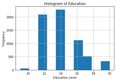

# histogram of marriage rating
dta.rateMarriage.hist()
plt.title('Histogram of Marriage Rating')
plt.xlabel('Marriage Rating')
plt.ylabel('Frequency')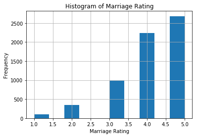

Let’s take a look at the distribution of marriage ratings for women having affairs, versus those having no affairs.

pd.crosstab(dta.rateMarriage, dta.affair.astype(bool)).plot(kind='bar')
plt.title('Marriage Rating Distribution by Affair Status')
plt.xlabel('Marriage Rating')
plt.ylabel('Frequency')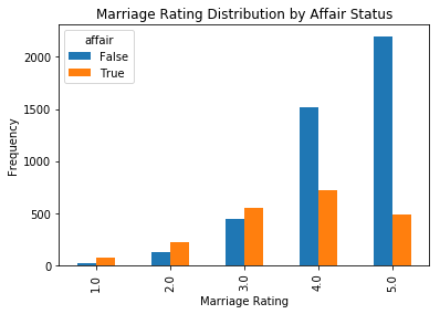

Let’s use a stacked bar-plot to look at the percentage of women having affairs by number of years of marriage.

affair_yrs_married = pd.crosstab(dta.yearsMmarried, dta.affair.astype(bool))
affair_yrs_married.div(affair_yrs_married.sum(1).astype(float), axis=0).plot(kind='bar', stacked=True)
plt.title('Affair Percentage by Years Married')
plt.xlabel('Years Married')
plt.ylabel('Percentage')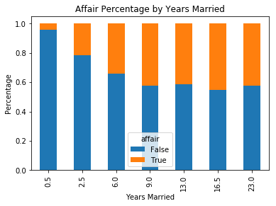

Prepare Data for Logistic Regression

To prepare the data, I want to add an intercept column as well as dummy variables for occupation and occupation_husb, since I’m treating them as categorical variables. The dmatrices function from patsy module can do that using formula language.

# create dataframes with an intercept column and dummy variables for
# occupation and occupation_husb
y, X = dmatrices('affair ~ rateMarriage + age + yearsMarried + children + \
                  religious + educ + C(occupation) + C(husbandOccupation)',
                  dta, return_type="dataframe")
X.columns
X.head(5)

	Intercept	C(occupation)[T.2.0]	C(occupation)[T.3.0]	C(occupation)[T.4.0]	C(occupation)[T.5.0]	C(occupation)[T.6.0]	C(husbandOccupation)[T.2.0]	C(husbandOccupation)[T.3.0]	C(husbandOccupation)[T.4.0]	C(husbandOccupation)[T.5.0]	C(husbandOccupation)[T.6.0]	rateMarriage	age	yearsMarried	children	religious	educ
0	1.0	1.0	0.0	0.0	0.0	0.0	0.0	0.0	0.0	1.0	0.0	3.0	32.0	9.0	3.0	3.0	17.0
1	1.0	0.0	1.0	0.0	0.0	0.0	0.0	0.0	1.0	0.0	0.0	3.0	27.0	13.0	3.0	1.0	14.0
2	1.0	0.0	1.0	0.0	0.0	0.0	0.0	0.0	0.0	1.0	0.0	4.0	22.0	2.5	0.0	1.0	16.0
3	1.0	0.0	0.0	0.0	1.0	0.0	0.0	0.0	0.0	1.0	0.0	4.0	37.0	16.5	4.0	3.0	16.0
4	1.0	0.0	1.0	0.0	0.0	0.0	0.0	0.0	1.0	0.0	0.0	5.0	27.0	9.0	1.0	1.0	14.0

The column names for the dummy variables are not intuitive, so let’s rename those.

# fix column names of X
X = X.rename(columns = {'C(occupation)[T.2.0]':'occ_2',
                        'C(occupation)[T.3.0]':'occ_3',
                        'C(occupation)[T.4.0]':'occ_4',
                        'C(occupation)[T.5.0]':'occ_5',
                        'C(occupation)[T.6.0]':'occ_6',
                        'C(husbandOccupation)[T.2.0]':'occ_husb_2',
                        'C(husbandOccupation)[T.3.0]':'occ_husb_3',
                        'C(husbandOccupation)[T.4.0]':'occ_husb_4',
                        'C(husbandOccupation)[T.5.0]':'occ_husb_5',
                        'C(husbandOccupation)[T.6.0]':'occ_husb_6'})



X.head()

	Intercept	occ_2	occ_3	occ_4	occ_5	occ_6	occ_husb_2	occ_husb_3	occ_husb_4	occ_husb_5	occ_husb_6	rateMarriage	age	yearsMarried	children	religious	educ
0	1.0	1.0	0.0	0.0	0.0	0.0	0.0	0.0	0.0	1.0	0.0	3.0	32.0	9.0	3.0	3.0	17.0
1	1.0	0.0	1.0	0.0	0.0	0.0	0.0	0.0	1.0	0.0	0.0	3.0	27.0	13.0	3.0	1.0	14.0
2	1.0	0.0	1.0	0.0	0.0	0.0	0.0	0.0	0.0	1.0	0.0	4.0	22.0	2.5	0.0	1.0	16.0
3	1.0	0.0	0.0	0.0	1.0	0.0	0.0	0.0	0.0	1.0	0.0	4.0	37.0	16.5	4.0	3.0	16.0
4	1.0	0.0	1.0	0.0	0.0	0.0	0.0	0.0	1.0	0.0	0.0	5.0	27.0	9.0	1.0	1.0	14.0

We also need to flatten y into a 1-D array, so that scikit-learn will understand it as response variable.

# flatten y into a 1-D array
y = np.ravel(y)

Logistic Regression

Let’s run logistic regression on the entire data set, and see how accurate it works!

model = LogisticRegression()
model = model.fit(X, y)

#accuracy obtained from training dataset
model.score(X, y)

0.7258875274897895

73% accuracy is good, but what about the null error rate?

# what percentage had affairs?
y.mean()

0.3224945020420987

Only 32% of the women had affairs, which means that the model can obtain 68% accuracy by always predicting “no”. So we’re doing better than the null error rate, but not much.

Let’s examine the coefficients to see what we learn.

# examine the coefficients
X.columns, np.transpose(model.coef_)

(Index(['Intercept', 'C(occupation)[T.2.0]', 'C(occupation)[T.3.0]',
        'C(occupation)[T.4.0]', 'C(occupation)[T.5.0]', 'C(occupation)[T.6.0]',
        'C(occupation_husb)[T.2.0]', 'C(occupation_husb)[T.3.0]',
        'C(occupation_husb)[T.4.0]', 'C(occupation_husb)[T.5.0]',
        'C(occupation_husb)[T.6.0]', 'rateMarriage', 'age', 'yearsMarried',
        'children', 'religious', 'educ'],
       dtype='object'),
 array([[ 1.42616802],
        [ 0.06677903],
        [ 0.37876591],
        [ 0.13853096],
        [ 0.79779521],
        [ 0.24306937],
        [ 0.31206687],
        [ 0.45477631],
        [ 0.26190426],
        [ 0.27958124],
        [ 0.24901274],
        [-0.70325862],
        [-0.05571589],
        [ 0.10585439],
        [ 0.00203596],
        [-0.36038626],
        [ 0.00652453]]))

Increases in marriage rating and religiousness corresponds to decrease in the likelihood of having an affair. For both, wife’s occupation and the husband’s occupation, the lowest likelihood of having an affair corresponds to the baseline occupation (student), since all of the dummy coefficients are positive.

Model Evaluation Using a Validation Set

So far, we have trained and tested on the same set. Let’s instead split the data into a training and a test set.

# evaluate the model by splitting the data-set into train and test sets
X_train, X_test, y_train, y_test = split(X, y, test_size=0.3)

model2 = LogisticRegression()
model2.fit(X_train, y_train)

We need to predict class labels for the test set. We will also generate the class probabilities, just take a look.

predicted = model2.predict(X_test)
print(y_test)
predicted

[0. 0. 0. ... 0. 0. 1.]
array([1., 0., 0., ..., 0., 0., 0.])

# generate class probabilities
probs = model2.predict_proba(X_test)
probs

array([[0.35891094, 0.64108906],
       [0.90821603, 0.09178397],
       [0.71072968, 0.28927032],
       ...,
       [0.53524571, 0.46475429],
       [0.82037132, 0.17962868],
       [0.74477992, 0.25522008]])

As you can see, the classifier is predicting 1 (having an affair) any time the probability in second column is greater than 0.5.

Now let’s generate some evaluation metrics.

# generate evaluation metrics
print(metrics.accuracy_score(y_test, predicted))
print(metrics.roc_auc_score(y_test, probs[:, 1]))

0.7335078534031414
0.7452425716348409

The accuracy is 73%, which is the same as we obtained when training and predicting on the same data.

We can see the confusion matrix and a classification report with other metrics.

import seaborn as sns
conf_matrix = metrics.confusion_matrix(y_test, predicted)
sns.heatmap(conf_matrix, annot=True,cmap='Blues')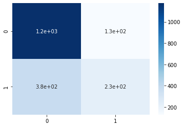

print(metrics.classification_report(y_test, predicted))

              precision    recall  f1-score   support

         0.0       0.76      0.90      0.82      1303
         1.0       0.64      0.37      0.47       607

    accuracy                           0.73      1910
   macro avg       0.70      0.64      0.65      1910
weighted avg       0.72      0.73      0.71      1910

Model Evaluation Using Cross-Validation

Now let’s use 10-fold cross-validation, to see if the accuracy holds up more rigorously.

# evaluate the model using 10-fold cross-validation
scores = cross_val_score(LogisticRegression(), X, y, scoring='accuracy', cv=10)
scores, scores.mean()

(array([0.72100313, 0.70219436, 0.73824451, 0.70597484, 0.70597484,
        0.72955975, 0.7327044 , 0.70440252, 0.75157233, 0.75      ]),
 0.7241630685514876)

Looks good. It’s still performing at 73% accuracy.

Final Thoughts

We have developed a classification model using Logistic Regression and got a decent accuracy of 73%. We can perform hyper-parameter tuning to get better accuracy out of the model. I will leave it for the readers to do some tuning and make it more accurate. In my next blog, I will be writing about unsupervised machine learning algorithms and implement them in Python.