
Data Pre-processing in Python
Preparation is the basic need to complete a task with near perfection, whether be it a football match or an online exam. Someone has to take a lot of preparation before they can achieve perfect result. In the same way, preparing the data before modeling and doing exploratory data analysis, is the basic task that needs to be done by every data science professionals to get accurate results. Here in this blog post I am going to discuss in details about preparing a data-set before finding interesting insights.
What is the need of pre-processing?
When we deal with real world data, there are lots of inconsistency such as:
Incomplete data: Missing values due to improper collection of data
Noisy data: Outliers or errors introduced while collecting data
The data-set may be imbalanced, i.e. for example, for a classification task, the data-set has more data for a positive class than negative class. If we train a machine learning model using this imbalanced data, the prediction might always be biased towards abundant class since it did not get trained properly on the rare class. So we have to make the data-set balanced before modelling.
Data pre-processing is required to remove all the inconsistency in the dataset and make it into an efficient format before it can be used for analysis. I am going to go step by step about pre-processing the dataset using Melbourne Housing Dataset.
Steps involved in pre-processing
Let us start the pre-processing steps by loading the python packages and the dataset.
#import the required libraries
import pandas as pd
import numpy as np
#loading the dataset and viewing the first 5 columns
original_df = pd.read_csv('S:/media/melb_data.csv')
original_df.shape(13580, 21)We can see there are 13580 rows and 21 columns in our data-set. Let us visualize five random rows in the data-set.
original_df.sample(5)| Suburb | Address | Rooms | Type | Price | Method | SellerG | Date | Distance | Postcode | … | Bathroom | Car | Landsize | BuildingArea | YearBuilt | CouncilArea | Lattitude | Longtitude | Regionname | Propertycount | |
|---|---|---|---|---|---|---|---|---|---|---|---|---|---|---|---|---|---|---|---|---|---|
| 4081 | Moonee Ponds | 6/7 York St | 1 | u | 360000.0 | SP | Brad | 10/12/2016 | 6.9 | 3039.0 | … | 1.0 | 1.0 | 0.0 | 54.0 | 1965.0 | Moonee Valley | -37.76520 | 144.91160 | Western Metropolitan | 6232.0 |
| 8937 | Rowville | 11 Jindalee Cl | 5 | h | 870000.0 | S | Harcourts | 1/07/2017 | 23.5 | 3178.0 | … | 2.0 | 2.0 | 733.0 | 217.0 | 1986.0 | Knox | -37.91894 | 145.24305 | South-Eastern Metropolitan | 11667.0 |
| 3473 | Keilor East | 564 Buckley St | 3 | h | 630000.0 | S | Nelson | 16/04/2016 | 12.8 | 3033.0 | … | 2.0 | 1.0 | 221.0 | NaN | NaN | Moonee Valley | -37.75040 | 144.85940 | Western Metropolitan | 5629.0 |
| 9115 | Craigieburn | 195 Newbury Bvd | 4 | h | 667000.0 | S | Ray | 3/06/2017 | 20.6 | 3064.0 | … | 2.0 | 2.0 | 480.0 | 214.0 | 2012.0 | Hume | -37.57201 | 144.90897 | Northern Metropolitan | 15510.0 |
| 5405 | Richmond | 22a Stanley St | 3 | h | 1600000.0 | S | Biggin | 24/09/2016 | 2.6 | 3121.0 | … | 2.0 | 2.0 | 80.0 | 144.0 | 1850.0 | Yarra | -37.82330 | 144.99470 | Northern Metropolitan | 14949.0 |
5 rows × 21 columns
It is evident from the data-set that there are missing values in “BuildingArea” and “YearBuilt” column as “Nan” values are present. Let us check number of missing values in every column of the entire data-set.
#the below code counts the number of missing values in each column
original_df.isna().sum()
Suburb 0
Address 0
Rooms 0
Type 0
Price 0
Method 0
SellerG 0
Date 0
Distance 0
Postcode 0
Bedroom2 0
Bathroom 0
Car 62
Landsize 0
BuildingArea 6450
YearBuilt 5375
CouncilArea 1369
Lattitude 0
Longtitude 0
Regionname 0
Propertycount 0
dtype: int64We can see that “Car”,”BuildingArea”,”YearBuilt” and “CouncilArea” definitely has missing values. Now there are 3 options to handling of missing values.
- Drop the columns with missing value: This is very simple approach and is not recommended as lots of “important” information can be lost by simply dropping the columns. Missing columns can be dropped by
dataset_without_missing_column = original_df.dropna(axis=1)
dataset_without_missing_column.isna().sum()
Suburb 0
Address 0
Rooms 0
Type 0
Price 0
Method 0
SellerG 0
Date 0
Distance 0
Postcode 0
Bedroom2 0
Bathroom 0
Landsize 0
Lattitude 0
Longtitude 0
Regionname 0
Propertycount 0
dtype: int64We can see the columns having missing values are dropped and now the data-set has no missing values. Now lets look at the next option.
- Drop the rows with missing value: This is another very simple approach and is not recommended as again, lots of “important” information can be lost. Rows with missing values can be dropped by
dataset_without_missing_row = original_df.dropna()
dataset_without_missing_row.isna().sum()
Suburb 0
Address 0
Rooms 0
Type 0
Price 0
Method 0
SellerG 0
Date 0
Distance 0
Postcode 0
Bedroom2 0
Bathroom 0
Car 0
Landsize 0
BuildingArea 0
YearBuilt 0
CouncilArea 0
Lattitude 0
Longtitude 0
Regionname 0
Propertycount 0
dtype: int64We can see that there are no missing values in the dataset. This approach is suitable when there are lots of data in the dataset. Let us look at the 3rd option
- Imputation: As the name suggests, we can impute values in the data-set to replace the missing values. This kind of approach tends to work out well. Imputation is the process of replacing the missing values with mean or median values , in case of numerical columns and mode values, in case of categorical columns. Let me use Scikit-learn’s SimpleImputer class to impute mean values in the numerical columns.
from sklearn.impute import SimpleImputer
imputer = SimpleImputer()
imputed_numerical = imputer.fit_transform(original_df.select_dtypes(exclude=['object']))
imputed_numerical = pd.DataFrame(imputed_numerical, columns=original_df.select_dtypes(exclude=['object']).columns)
imputed_numerical.isna().sum()
Rooms 0
Price 0
Distance 0
Postcode 0
Bedroom2 0
Bathroom 0
Car 0
Landsize 0
BuildingArea 0
YearBuilt 0
Lattitude 0
Longtitude 0
Propertycount 0
dtype: int64We can see that the numerical columns are imputed and no missing values are found. Lets see how the categorical columns can be imputed
imputer = SimpleImputer(strategy="most_frequent")
imputed_categorical = imputer.fit_transform(original_df.select_dtypes(include=['object']))
imputed_categorical = pd.DataFrame(imputed_categorical, columns = original_df.select_dtypes(include=['object']).columns)
imputed_categorical.isna().sum()
Suburb 0
Address 0
Type 0
Method 0
SellerG 0
Date 0
CouncilArea 0
Regionname 0
dtype: int64Here we can see, the categorical columns are imputed with most frequent,i.e., mode of the column.
In the above discussion, we have only used mean and mode imputation. There are lots of complex imputation techniques but it has been observed that simple is always better than complex and the complex imputation techniques doesn’t achieve high accuracy as desired. So we will stop our discussion on missing value treatment and move on to Feature Scaling.
Feature Scaling
Feature scaling is a very important task that needs to be done during pre-processing of the data-set. Feature scaling is the method by which independent variables(predictors) are scaled to a standardized value. There are mainly 2 ways we can do that, Min-Max Normalization and Standardization.
Min-Max Normalization
It is the simplest method and it re-scales the data in range between 0 and 1. Here is the formula for min-max normalization
x’ = (x – min(x))/(max(x)-min(x))
Let us apply min-max normalization in python and visualize the data-set.
#create a simple pandas dataframe
s1 = pd.Series([1, 2, 3, 4, 5, 6, 7], index=(range(7)))
s2 = pd.Series([10, 9, 8, 7, 6, 5, 4], index=(range(7)))
s3 = pd.Series([100,200,300,500,500,789,458], index=(range(7)))
df = pd.DataFrame({'s1': s1,'s2':s2,'s3':s3})
df
| s1 | s2 | s3 | |
|---|---|---|---|
| 0 | 1 | 10 | 100 |
| 1 | 2 | 9 | 200 |
| 2 | 3 | 8 | 300 |
| 3 | 4 | 7 | 500 |
| 4 | 5 | 6 | 500 |
| 5 | 6 | 5 | 789 |
| 6 | 7 | 4 | 458 |
We created a simple data-set which has different range of values. Let us apply min-max normalization.
from mlxtend.preprocessing import minmax_scaling

min_max_normalized = minmax_scaling(df, columns=df.columns)
min_max_normalized| s1 | s2 | s3 | |
|---|---|---|---|
| 0 | 0.000000 | 1.000000 | 0.000000 |
| 1 | 0.166667 | 0.833333 | 0.145138 |
| 2 | 0.333333 | 0.666667 | 0.290276 |
| 3 | 0.500000 | 0.500000 | 0.580552 |
| 4 | 0.666667 | 0.333333 | 0.580552 |
| 5 | 0.833333 | 0.166667 | 1.000000 |
| 6 | 1.000000 | 0.000000 | 0.519594 |
min_max_normalized.describe()| s1 | s2 | s3 | |
|---|---|---|---|
| count | 7.000000 | 7.000000 | 7.000000 |
| mean | 0.500000 | 0.500000 | 0.445159 |
| std | 0.360041 | 0.360041 | 0.332220 |
| min | 0.000000 | 0.000000 | 0.000000 |
| 25% | 0.250000 | 0.250000 | 0.217707 |
| 50% | 0.500000 | 0.500000 | 0.519594 |
| 75% | 0.750000 | 0.750000 | 0.580552 |
| max | 1.000000 | 1.000000 | 1.000000 |
We can see that the data-set has been scaled in the range of 0 and 1.
Standardization
Standardization is a method to re-scale the data-set to have zero mean and 1 standard deviation. It is also called z-score normalization. Let us apply standardization on the simple data-set that we created above.
from mlxtend.preprocessing import standardize

standardized = standardize(df,columns=df.columns)
standardized| s1 | s2 | s3 | |
|---|---|---|---|
| 0 | -1.5 | 1.5 | -1.447314 |
| 1 | -1.0 | 1.0 | -0.975437 |
| 2 | -0.5 | 0.5 | -0.503560 |
| 3 | 0.0 | 0.0 | 0.440194 |
| 4 | 0.5 | -0.5 | 0.440194 |
| 5 | 1.0 | -1.0 | 1.803919 |
| 6 | 1.5 | -1.5 | 0.242006 |
standardized.describe()| s1 | s2 | s3 | |
|---|---|---|---|
| count | 7.000000 | 7.000000 | 7.000000e+00 |
| mean | 0.000000 | 0.000000 | -2.775558e-17 |
| std | 1.080123 | 1.080123 | 1.080123e+00 |
| min | -1.500000 | -1.500000 | -1.447314e+00 |
| 25% | -0.750000 | -0.750000 | -7.394988e-01 |
| 50% | 0.000000 | 0.000000 | 2.420055e-01 |
| 75% | 0.750000 | 0.750000 | 4.401939e-01 |
| max | 1.500000 | 1.500000 | 1.803919e+00 |
We can see that all the columns has mean 0 and standard deviation approximately 1.
Standardization and normalization are important concepts and should be used before modelling. Let me now discuss about another important concept, Handling of Imbalanced data-set.
Imbalanced data-set
As the name suggests, an imbalanced dataset is something that has lots of example for a particular class and very less example for other class. So, when we are modelling a classification model, using this dataset, we can get very high accuracy for the particular class but very less accuracy for the other. This means the model cannot generalize well and it is very biased towards the particular class. So we have to handle this problem, i.e., we have to make the dataset a balanced one and then use it for modelling.
There are two ways to make a dataset balanced, under-sampling and over-sampling of dataset.
- Under-sampling: Under-sampling is a technique to reduce the number of examples in the abundant class by randomly selecting the rows belonging to that class. All the samples in the rare class are kept intact. It is used when the data-set is large enough to have lots of data.
- Over-sampling: In this technique, the rare samples are generated using repetition, boot-strapping or SMOTE(Synthetic Minority Over-Sampling Technique). In this way number of rare samples is increased in the data-set and can be balanced.
There is absolutely no advantage of one sampling technique with other. It all depends on the use-case and the dataset we are working in.
Let us see in python how we can use these techniques to balance-scale dataset
imbalanced_df = pd.read_csv('S:/xxxx/balance-scale.data',names=['balance', 'v1', 'v2', 'v3', 'v4'])
imbalanced_df.shape
(625, 5)The data-set has 625 rows and 5 columns. Let us look at first 5 rows of the data-set
imbalanced_df['balance'].value_counts()R 288
L 288
B 49
Name: balance, dtype: int64imbalanced_df['balance'].value_counts().plot(kind='bar')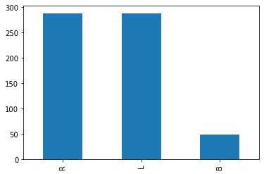
We can see that the dataset is imbalanced with “B” being the rare class. Lets make a logistic regression model using this dataset
from sklearn.linear_model import LogisticRegression
from sklearn.metrics import accuracy_score
# Separate predictor features (X) and target (y)
y = imbalanced_df.balance
X = imbalanced_df.drop('balance', axis=1)

# Train model
logistic_regression_model = LogisticRegression().fit(X, y)

# Predict on training set
pred_imbalanced = logistic_regression_model.predict(X)

# Lets look at the accuracy?
print( accuracy_score(pred_imbalanced, y) )0.8848from sklearn.metrics import confusion_matrix
import seaborn as sns
conf_matrix = confusion_matrix(y, pred_imbalanced)
sns.heatmap(conf_matrix, annot=True,cmap='Blues')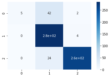
From the confusion matrix, it can be visualized that “B” class denoted by “0” is not getting predicted properly. Only 5 samples got proper prediction out of 49. So it is evident that the model is not performing well. Let us now balance the data-set using over-sampling the data-set.
from sklearn.utils import resample
#Separate majority and minority classes
df_major = imbalanced_df[imbalanced_df.balance.isin(['L','R'])]
df_minor = imbalanced_df[imbalanced_df.balance=='B']
# Upsample minority class
df_minor_oversampled = resample(df_minor, replace=True, n_samples=288,random_state=123)
# Combine the majority class with upsampled minority class

df_oversampled = pd.concat ([df_major, df_minor_oversampled])
# Display new class counts
df_oversampled.balance.value_counts()
L    288
B    288
R    288
Name: balance, dtype: int64
# Separate predictor features (X) and target (y)
y = df_oversampled.balance
X = df_oversampled.drop('balance', axis=1)
# Train model
logistic_regression_model = LogisticRegression().fit(X, y)
# Predict on training set
pred_balanced = logistic_regression_model.predict(X)# Lets look at the accuracy?
print( accuracy_score(pred_balanced, y) )conf_matrix = confusion_matrix(y, pred_balanced)
sns.heatmap(conf_matrix, annot=True,cmap='Blues')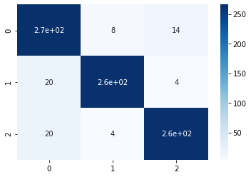
We can see that the model accuracy has increased as well as from the confusion matrix, it is evident that the model can generalize well. Since we do not have much data, it will be impractical to apply under-sampling, so we will skip that step here. You can definitely try that and let me know how did it perform.
Final Thoughts – Data Pre-Processing using Python
Here in this blog I tried to discuss in detail about data pre-processing and handling of imbalanced data-set. These are the basic task that needs to be performed by a data science professional, on their day to day work. In my next blog, I will be writing about Exploratory Data Analysis and find out interesting insights from there. Please stay tuned for further updates.

