Control Structures in R Programming
What are Control Structures?
Control Structures are an integral part of any programming language. We can say that a programming language without control structures is incomplete. These control structures are basically a block of code lines that decide which direction to go once the executed and often called as well as considered as loops. Control structures are mostly used for decision making.
Under R programming as well, we find different control structures which decide the execution of the code blocks. We can use these control structures as sole or in combination with each other to get the desired control of programming flow. R Provides around eight of the control structures as listed below. We will discuss each one of them in detail throughout this article.
Control Structures in R Programming
- If – else statement
- ifelse() function
- Switch Statement
- for loop
- while loop
- Break Statement
- Next Statement
- Report Loops
Let’s discuss these control structures one by one throughout this article.
If – else Statement in R Programming
If – else is an important statement in R, which can be categorized under conditional statements which allows to enhance the conditional execution of a block of code in R. If – else statement plays an important role under in decision making under R and allows us to make decisions based on whether the condition is satisfied (i.e. TRUE) or not satisfied (i.e. FALSE). The working of If – else is pretty much simple.
- The
ifstatement contains a logical condition that needs to be evaluated and checked. There is a block of code underifstatement which gets executed and returns output once the logical condition is satisfied or is TRUE. Otherwise, if the logical condition doesn’t get satisfied or is FALSE, the block of code does not get executed. - Then comes the
elsepart of this statement. This part allows us to execute a block of code when the logical condition mapped under theifstatement gives output as FALSE.
However, in R, we have a luxury to use the conditional if statement as sole as well. If the condition gets satisfied, the system will execute the block of code. Otherwise it will not execute the same. Let’s run out some examples to have a better understanding.
> #Using logical if statement

> x <- 3      #Defining a variable x
> y <- 6      #Defining a variable y

> if(x<y){                           #Checking logical condition whether x < y
+   print("x is smaller than y")     #Block of code to execute if logical condition is True
+ }
[1] "x is smaller than y"            #Output
In the example above, we have defined two variables x and y with values 3 and 6 respectively. We have a logical condition to check whether x is less than y or not. If the logical condition holds, a block of code under the curly braces ({}) should get executed. Remember that every control structure and conditional statement in R uses curly braces to specify the arguments (block of code to execute) under them. Once we run the code above, the system first checks whether the logical condition holds (it holds here) and then prints a statement "x is smaller than y".
Now, we will see how an else statement can be added to execute an alternative block of code which should be printed when condition under the if statement doesn’t hold.
> #Using logical if statement

> x <- 3         #defining a variable x
> y <- 6         #defining a variable y

> if(x > y){                      #Logical condition to be tested
+   print("x is greater than y")  #block of code to be executed when if condition holds
+ } else {
+   print("y is greater than x")  #block of code to be executed when if condition doesn't
                                                                                  hold
+ }
[1] "y is greater than x"         #output
Here, we are trying to check whether the logical condition holds. Since x is not greater than y, the logical condition doesn’t hold and hence we need to add another block of code under else statement which should print a statement y is greater than x.
We can also specify multiple logical conditions under one code to get the different blocks of the code being executed. we have else if statement to achieve this result. This procedure of adding multiple if conditions in your program is also known as nesting of the if-else statements. Please see an example below for a better understanding.
> # nested if-else
> x <- -4                            #Defining a variable x with value as -4

> if (x > 0){                        #First logical condition
+   print("x is a positive number")  #block of code for first logical condition
+ } else if (x < 0) {                #Second logical condition
+   print("x is a negative number")  #block of code for second logical condition
+ } else {
+   print("value for x is zero")     #block of code for else statement
+ }
[1] "x is a negative number"         #output
we have first created a variable named x and assigned value as -4 to it. The first if statement checks if the value assigned to x is greater than zero or not. If it is greater than zero, x is a positive number gets printed out. the second logical condition gets checked under else if statement for whether x is less than zero or not. If it is less than zero, x is a negative number gets printed out. Finally, if both the logical conditions don’t hold, the final block of code gets printed out which is under else statement and reads as value for x is zero.
ifelse() Function in R Programming
Unlike if – else statement, we also have ifelse() function under R which works in the same manner as the if – else statement does. The reason for it to introduce under R is quite related to the speed. Since most of the functions take a vector/s as an argument/s and it is quite a speedy procedure to check the condition based on a vector under a function rather than checking it under if – else statement. As discussed earlier it genuinely works as the same as if – else do. This function can be used in the same way we use logical IF conditions under Microsoft Excel.
Syntax for ifelse() function is as shown below:
ifelse(test, True, False)
Where –
test– is a logical test/condition that we need to check and which either holds or not.True– symbolizes the expression that gets evaluated if the condition provided under test holdsFalse– symbolizes the expression that gets evaluated if the condition provided doesn’t hold.
Let’s see an example to walk through the concept more precisely.
> #Working with ifelse function

> z <- 12

> #using ifelse() function to check the condition and get output accordingly

> ifelse(z <= 10, "z is less than or equals to 10", "z is greater than 10")

[1] "z is greater 10"                       #Output
In the example above, we have defined a variable z with value 12 assigned to it. under the ifelse() function, we are trying to check whether z is less than or equals to 10. If this test holds, we are specifying an output to be printed as z is less than or equals to 10. If this test doesn’t hold (as in our case), the output should be z is greater than 10 (which ideally is our output).
Let’s move towards the next control structure from the list: switch statement.
Switch Statement in R Programming
It can be a hard way for someone to write multiple if-else statements for different alternatives for a condition. Instead of that, we have a statement named switch which allows us to specify a value or condition as an argument under it and generates the result based on the value or condition specified. each possible alternative under switch is called a case. Following is the syntax for the switch statement in R.
switch(Exp, case1, case2, case3, ...)
Where-
Exp– specifies the expression to be added as an argument under the switch statement.case1, case2, case3, ...– set of alternatives out of which a one will be gets printed as an output based on the value of Exp.
Go through the example below for a better understanding of switch in R.
> #Working with switch statement in R

> p <- 3                              #Defining a variable p with value as 3

>#Specifying multiple cases based on the argument value under Switch

> switch(p,
+        "This is the first value under switch",
+        "This is the second value under switch",
+        "This is the third value under switch",
+        "This is the fourth value under switch",
+        "This is the fifth value under switch")

[1] "This is the third value under switch"   #Output
We first have created a variable named p with the value assigned to it as 3. Under the switch statement, we have used this p as an argument and have added five cases out of which one should hold and get printed out as an output based on the value of p. Since the value of p is 3, we get the third case printed out as an output that reads as This is the third value under switch.
This is how the switch statement work under R. We will head towards the next and one of the most important control structure in R, a “for loop”.
for Loops in R Programming
Looping or iterating is a concept we are all well versed and is widely used in all programming languages. It has origin even before the computer programming languages were invented or developed. The most basic loop structure in any programming language is a for loop. So does it in R.
The for loop is a structure that allows us to repeat/iterate some block of codes based on the sequences provided as an argument under the loop body. It iterates/loops the block of code as soon as the argument holds. The argument most of the time is a sequential vector(or variable). following is a syntax associated with the for loop.
for (variable_in_sequence) {
     Expressions_to_repeat
    }
Where –
variable_in_sequence– specifies the sequential variable that is used as a condition under for loop to iterate the block of code.Expressions_to_repeat– specifies the expressions that are supposed to be repeated until we reach the last value ofvariable_in_sequence.
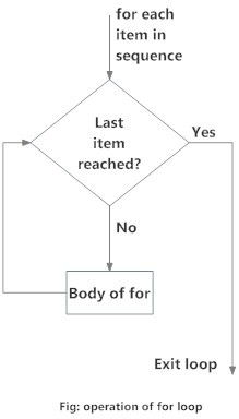
We can also map a flow chart associated with for loop as shown below.
source of image: https://cdn.datamentor.io/wp-content/uploads/2017/11/r-for-loop.jpg
In the flowchart image above, we can see one diamond block and one rectangle block. Diamond box stands for the decision making statements box or simply conditions box. The rectangle box is specified with all the expressions which are needed to be executed every time the decision box holds. for each item within the sequence provided, we check whether the last item is reached (conditions box). If it holds, the loop will be terminated. However, until it holds, the expressions under the rectangular box will be executed again and again.
Let’s take an example to have a better understanding of working of for loop.
> a <- LETTERS[1:10]             #Vector of first 10 elements of constants named LETTERS
>
> for(i in a){
+   print(i)                     #Printing each element of vector "a" as long as we reach
                                  the end of vector "a".
+ }
[1] "A"                          #Output
[1] "B"
[1] "C"
[1] "D"
[1] "E"
[1] "F"
[1] "G"
[1] "H"
[1] "I"
[1] "J"
We, in this example, has taken a subset (only 10 elements) of a built-in list of constants named “LETTERS” that consist of all the 26 roman alphabet in upper case. Under for loop, we are printing each of these elements from vector until we reach the last element of the vector. Thus we are getting an output ranged from A to J.
Final Words – Control Structures in R Programming
We will end this article here and try to cover the remaining four control structures in the next article in this series. If you feel this article has helped you through the concept of control structures in R, you can share your support through likes and positive comments through the comment section. You can also keep your doubts and questions posted related to this topic through the comment section and I will try to answer as much as I could.
Stay tuned for our next article in this series. Until then Stay Home! Stay Safe! 🙂

